
NBA Draft Pick Value by Draft Slot
There have been a number of times recently where I’ve wanted to look up an analysis of draft pick value by slot, and haven’t been able to find one, or been dissatisfied with the methodology or data that I found. So I decided to do one myself and write it up, while going into some depth on my reasoning and alternative ways to look at draft value. I’ll also include the code I wrote for scraping the data and wrangling it, in case there are people who want to replicate and/or extend my analysis.
If you don’t care about the technical details and exposition, you can skip to the meat of the analysis here.
Project setup
Data sources
I considered a variety of metrics to estimate player value. Ultimately, I decided on VORP due to being the most available decent player estimator: cf. DARKO/RAPTOR/EPM/RAPM, all of which only have limited amounts of coverage in the past 20 years, and RPM, which has had some…questionable results lately1. VORP isn’t perfect, but it’s a reasonable metric, and this analysis is mostly useful for a broad understanding of value, not trying to parse specific cases of if player X is better than player Y. The best ability is availability, after all.
The other data source I needed was draft pick data; for that I just used Basketball-Reference, which is conveniently also where VORP is kept.
R or Python?
This tasks involved in this analysis (web scraping, data wrangling, and visualization) are things that both R and Python do well, so either would be suitable. For this post, I’ll use R, because there’s some neat capabilities in the purrr package I want to showcase – more on that later!
Scraping the data
Basketball-reference doesn’t have an API, so I’m going to have to scrape and clean the data from their webpages. To do this, I’ll use the rvest package for webscraping, and, since I’ll be accessing a lot of pages in succession, the polite package to make sure I’m scraping responsibly and in accordance with the site’s robots.txt file.
# Load web scraping packages
library(rvest)
library(polite)

# Load data wrangling packages
library(dplyr)
library(tidyr)
library(purrr)
library(stringr)
library(stringi)

# Load visualization packages
library(ggplot2)
Getting draft pick information
Basketball-reference stores draft data in pages like this one, one for each draft. The URLs for each draft follow the same format, so we can easily loop through the years 1996-2014 and scrape the draft page for the given year. We’re doing those years so that players in the dataset will all have had enough time that we can evaluate their early-career performance.
To do that, I wrote a function to scrape a given page, which we can then apply to a list of our target years using the map function from the purrr package. This pattern of programming – writing a function and applying it to a list – is the core of functional programming, a really powerful and flexible paradigm that underlies R. I like functional programming a lot and think it’s great for data analysis, since so much of data analysis follows the basic “take data, apply a function, apply another function, apply a third function, done” pattern.
get_draft <- function(year){
  url <- glue::glue('https://www.basketball-reference.com/draft/NBA_{year}.html')

  draft_page <- url %>%
    bow() %>% # Use polite functions instead of rvest::read_html()
    scrape()

  # Grab the link to the player page so we can access their stats easily later
  player_urls <- draft_page %>%
    html_nodes(".left") %>%
    html_nodes("a") %>%
    html_attr("href") %>%
    keep(~str_detect(., "^/players"))

  player_table <- draft_page %>%
    html_table(header = T) %>%
    pluck(1) %>% # Get the first table on the page, this is the draft table
    set_names(seq(1, dim(.)[2])) %>% # set temp names so R doesn't complain
    select(2, 4, 3, 6) %>%
    set_names(.[1,]) %>%
    slice(-1) %>% # this and the above line sets the first row as colnames
    mutate(year = year, .before = 1) %>%
    filter(Player != "Round 2", Player  != "", Player != "Player") %>%
    mutate(Player = stri_trans_general(Player, "Latin-ASCII"), # clean diacritics
           Yrs = as.numeric(Yrs),
           url = player_urls)

  return(player_table)
}

# draft_pos <- map_df(1996:2014, get_draft)
draft_pos <- readr::read_csv('draft_pos.csv')

head(draft_pos)
## # A tibble: 6 x 6
##    year    Pk Player              Tm      Yrs url
##   <dbl> <dbl> <chr>               <chr> <dbl> <chr>
## 1  1996     1 Allen Iverson       PHI      14 /players/i/iversal01.html
## 2  1996     2 Marcus Camby        TOR      17 /players/c/cambyma01.html
## 3  1996     3 Shareef Abdur-Rahim VAN      12 /players/a/abdursh01.html
## 4  1996     4 Stephon Marbury     MIL      13 /players/m/marbust01.html
## 5  1996     5 Ray Allen           MIN      18 /players/a/allenra02.html
## 6  1996     6 Antoine Walker      BOS      12 /players/w/walkean02.html
Observant readers will notice that we aren’t using rvest::read_html() to grab our data, but instead we’re using a couple of funny-sounding functions: bow and scrape. These functions, from the polite package, make sure that when you’re scraping web data, you’re doing it in a way that complies with the site owner’s wishes and doesn’t put undue strain on the site. If you’re just accessing one page once, they’re not particularly necessary, but I’d encourage their use for any project where you’re going to be accessing multiple pages or repeatedly hitting one page.
In addition to just grabbing the name of the player selected in each draft slot, I also grab the number of years they played in the league, to easily determine if they made the NBA or not (this will be NA for players who never made the league), and the URL to the player’s page, so that we know where to scrape their VORP numbers from.
Getting player VORP
Now that we have all our draft picks in one dataframe, we can go about getting their season-by-season value. Getting VORP per season is important, because we’re particularly concerned with production in a player’s early years when assessing draft pick value – it’s extremely rare that a player actually provides value2 in Years 10+ to the team that drafted him.
To do this, I used a nice little feature of R dataframes – you can have a column of dataframes inside another dataframe! I simply write a function to grab a player’s season-by-season VORP from his player page, and mutate my draft pick dataframe, adding a column that has all the dataframes I get from applying my get_player_VORP function to the column of URLs.
get_player_vorp <- function(draft_year, url, years){
  base <- 'https://www.basketball-reference.com'
  full_url <- paste0(base, url)

  ## This if statemtent is to account for players who never made the NBA (but who
  ## may still have bb-ref pages with G-Lg/Euro/Intl/etc. stats)
  if(is.na(years)){
    return(NA)
  }

  suppressWarnings(
    player_vorp <- full_url %>%
      bow() %>%
      scrape() %>%
      html_table(header = T) %>%
      keep(~"VORP" %in% colnames(.)) %>%
      pluck(1) %>% # above finds advanced stats tables, this picks the RS one
      select(1, 2, 3, 29) %>%
      mutate(Season = as.numeric(str_sub(Season, end = 4)) + 1) %>%
      filter(!is.na(Season)) %>%
      group_by(Season) %>%
      filter(n() == 1 | Tm == 'TOT') %>% # keep only season totals for split seasons
      ungroup() %>%
      mutate(year = draft_year,
             cyear = Season - year) %>%
      select(year, cyear, vorp = VORP)
  )

  return(player_vorp)
}

# draft_career <- draft_pos %>%
#   mutate(career_vorp = pmap(list('draft_year' = year,
#                                  'url' = url,
#                                  'years' = Yrs),
#                             get_player_vorp))

draft_career <- readr::read_rds('draft_career.rds')

head(draft_career)
## # A tibble: 6 x 5
##    year pk    player              team  data
##   <int> <chr> <chr>               <chr> <list>
## 1  1996 1     Allen Iverson       PHI   <tibble [20 x 2]>
## 2  1996 2     Marcus Camby        TOR   <tibble [21 x 2]>
## 3  1996 3     Shareef Abdur-Rahim VAN   <tibble [14 x 2]>
## 4  1996 4     Stephon Marbury     MIL   <tibble [17 x 2]>
## 5  1996 5     Ray Allen           MIN   <tibble [20 x 2]>
## 6  1996 6     Antoine Walker      BOS   <tibble [14 x 2]>
Initial analysis
So now that we have data, let’s start by getting an initial sense of what it looks like.
How valuable is a player to the team that drafts him?
As noted before, we want to focus on a player’s early-career value in this analysis, since almost all players will move on from the team that drafted them by the end of the period of team control.
Speaking of team control, it’s a useful lens for thinking about how to estimate draft pick value. Teams can sign contracts guaranteeing up to four years of direct team control3, and then control a player’s rights after that through restricted free agency. If a team wants to control a player’s rights, they have him under team control for a guaranteed four years, and then a reasonably good position to retain him for the next four. Thus, for this analysis, I’ll estimate a player’s value to the team that drafted him as the full value of his VORP for the first four years, plus half the value of his VORP for the next four.
Overall distribution of draft pick value
get_draft_value <- function(df){
  # Account for players who never made the league
  if(is.na(df$cyear[[1]])){
    return(-1.5)
  }

  else {
    cvorp <- df %>%
      summarize(VORP = sum(case_when(cyear <= 4 ~ VORP,
                                     cyear <= 8 ~ VORP*0.5,
                                     T~0))) %>%
      pull(VORP) %>%
      pluck(1)
  }

  return(cvorp)
}

draft_value <- draft_career %>%
  # map_dbl() is a map variant that converts the result to a vector of doubles
  mutate(value = map_dbl(data, get_draft_value),
         years = map_dbl(data, ~max(.$cyear))) %>%
  select(year, pk, team, player, years, value)

ggplot(draft_value %>%
         filter(!is.na(years))) +
  geom_histogram(aes(value), binwidth = 0.1, fill = '#C71400') +
  labs(x = 'Draft VORP', y = '# of players',
       title = 'Early career VORP of drafted players, 1996-2014',
       caption = 'Source: basketball-reference.com') +
  theme_bw() +
  theme(panel.border = element_blank(),
        panel.background = element_rect(fill = '#e4e5e2'),
        plot.background = element_rect(fill = '#e4e5e2'),
        plot.title = element_text(size = 18),
        axis.line = element_blank(),
        panel.grid = element_line(color = alpha('#555555', 0.1)),
        text = element_text(family = 'Gill Sans MT'))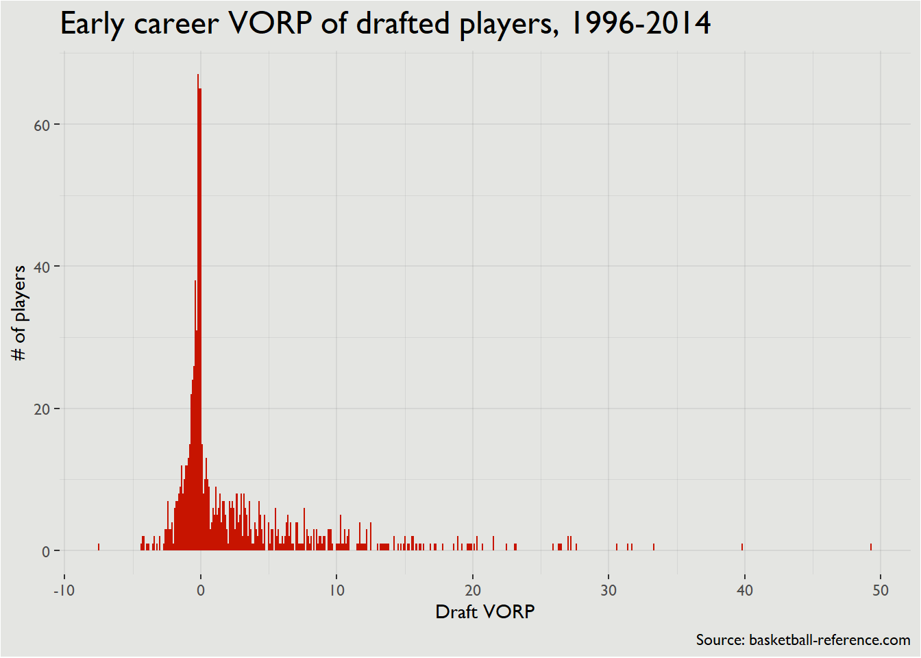
Breaking it down by role
I also think it’s useful to break a player’s value into categories by roles – we’ll use these roles again a bit later. For now, though, it’s interesting to not that there’s not a superstar-level player in about 20% of drafts, and there’s only 2-3 All-Star level players in an average draft.
draft_value %>%
  mutate(role = case_when(value >= 25 ~ "Superstar",
                          value >= 15 ~ "All-Star",
                          value >= 5 ~ "Starter",
                          value >= 0 ~ "Rotation",
                          value > -1.5 ~ "Bench",
                          T ~ "Sub-replacement"),
         # Order the factor, otherwise levels will be assigned alphabetically
         role = factor(role, levels = c("Superstar", "All-Star", "Starter",
                                        "Rotation", "Bench", "Sub-replacement"))) %>%
  group_by(role) %>%
  summarize(avg_per_draft = round(n()/length(unique(draft_value$year)), 2)) %>%
gt::gt()| role | avg_per_draft |
|---|---|
| Superstar | 0.79 |
| All-Star | 1.79 |
| Starter | 7.74 |
| Rotation | 17.21 |
| Bench | 19.00 |
| Sub-replacement | 12.42 |
How to think about value
Not pegging too closely to any particular pick
One of my original concerns when starting this project was not wanting to hew too closely to the picks that were made in any particular spot. Otherwise, you get obviously-not-useful results like the 41st pick having a higher average value than the 11th and 12th picks4.
The method I came up with is to average the value of the player picked in a particular spot with the value of other players the team could have taken (i.e., the players taken after him). Realistically, though, there are only so many players in consideration at any particular slot. It’s not like if the Cavs hadn’t taken Evan Mobley at #2 they would have potentially taken Cam Thomas or Luka Garza. So what I did is average the player with the picks a specified number of picks back: second round picks were averaged with the 5 picks back, since there’s a lot of variability in teams’ boards in the second round; non-lottery first-rounders were averaged with the three picks back; lottery picks, 2; all the way up to top-5 picks, who are averaged with the player behind them because of how tight boards typically are in that range.
What about players who never made the league?
One of the trickier questions in this analysis is how to deal with players who never made the NBA. In my opinion, removing them from the analysis, as most prior attempts do, does not fully capture the negative impact of drafting someone who never plays for you. The intuition here – unfortunately I haven’t been able to come up with a way to quantify this – is that young players who perform at a replacement player level (e.g. 0 VORP) are actually fairly valuable, since young players are generally quite bad. A rookie-contract player playing at that level would likely have reasonable trade value, certainly more than someone playing internationally or in the G-League who is not able/willing to come to the NBA.
Thus, I decided to assign players who never made the NBA a career value of -1.5, about equivalent to the worst player in the league over a given season, to roughly estimate the production of an equivalent player.
Value by pick
draft_value_by_pick <- draft_value %>%
  group_by(year) %>%
  mutate(pk = as.numeric(pk),
         num_picks = max(pk)) %>%
  ungroup() %>%
  mutate(pick_value = case_when(pk <= 5 ~ (value + lead(value, 1))/2,
                                pk <= 14 ~ (value + lead(value, 1) +
                                  lead(value, 2))/3,
                                pk <= 30 ~ (value + lead(value, 1) +
                                  lead(value, 2) + lead(value, 3))/4,
                                # Take the average of surrounding players for the
                                # last five picks in the draft
                                (num_picks - pk) >= 5 ~ (value + lead(value, 1) +
                                  lead(value, 2) + lead(value, 3) +
                                  lead(value, 4) + lead(value, 5))/6,
                                (num_picks - pk) == 4 ~ (value + lead(value, 1) +
                                  lead(value, 2) + lead(value, 3) +
                                  lead(value, 4) + lag(value, 1))/6,
                                (num_picks - pk) == 3 ~ (value + lead(value, 1) +
                                  lead(value, 2) + lead(value, 3) +
                                  lag(value, 2) + lag(value, 1))/6,
                                (num_picks - pk) == 2 ~ (value + lead(value, 1) +
                                  lead(value, 2) + lag(value, 3) +
                                  lag(value, 2) + lag(value, 1))/6,
                                (num_picks - pk) == 1 ~ (value + lead(value, 1) +
                                  lag(value, 4) + lag(value, 3) +
                                  lag(value, 2) + lag(value, 1))/6,
                                (num_picks - pk) == 0 ~ (value + lag(value, 1) +
                                  lag(value, 4) + lag(value, 3) +
                                  lag(value, 2) + lag(value, 1))/6)) %>%
  group_by(pk) %>%
  summarize(pk_value = mean(pick_value))

ggplot(draft_value_by_pick) +
  geom_col(aes(pk, pk_value), fill = '#C71400', width = .8) +
  # Highlight lottery
  annotate("area", x = c(0.5,14.5), y = 10, fill = 'black', alpha = .1) +
  annotate("text", x = 14, y = 10, label = 'Lottery',
           family = 'Gill Sans MT', hjust = 1, vjust = 1.2) +
  # Highlight 2nd round -- geom_area doesn't work here because values are + and -
  annotate("ribbon", x = c(30.5, 60.5), ymax = 2.5, ymin = -1,
           fill = 'black', alpha = .1) +
  annotate("text", x = 60, y = 2.5, label = '2nd Round',
           family = 'Gill Sans MT', hjust = 1, vjust = 1.2) +
  scale_x_continuous(breaks = c(1, seq(5, 60, 5))) +
  labs(x = 'Pick #', y = 'Mean early-career value available at slot',
       title = 'Average draft value by slot, 1996-2014',
       subtitle = 'Value is mean early-career VORP of players in consideration to be taken',
       caption = 'Data source: basketball-reference.com') +
  theme_bw() +
  theme(panel.border = element_blank(),
        panel.background = element_rect(fill = '#e4e5e2'),
        plot.background = element_rect(fill = '#e4e5e2'),
        plot.title = element_text(size = 18),
        plot.subtitle = element_text(color = 'gray50'),
        axis.line = element_blank(),
        panel.grid = element_line(color = alpha('#555555', 0.1)),
        panel.grid.minor.x = element_blank(),
        text = element_text(family = 'Gill Sans MT'))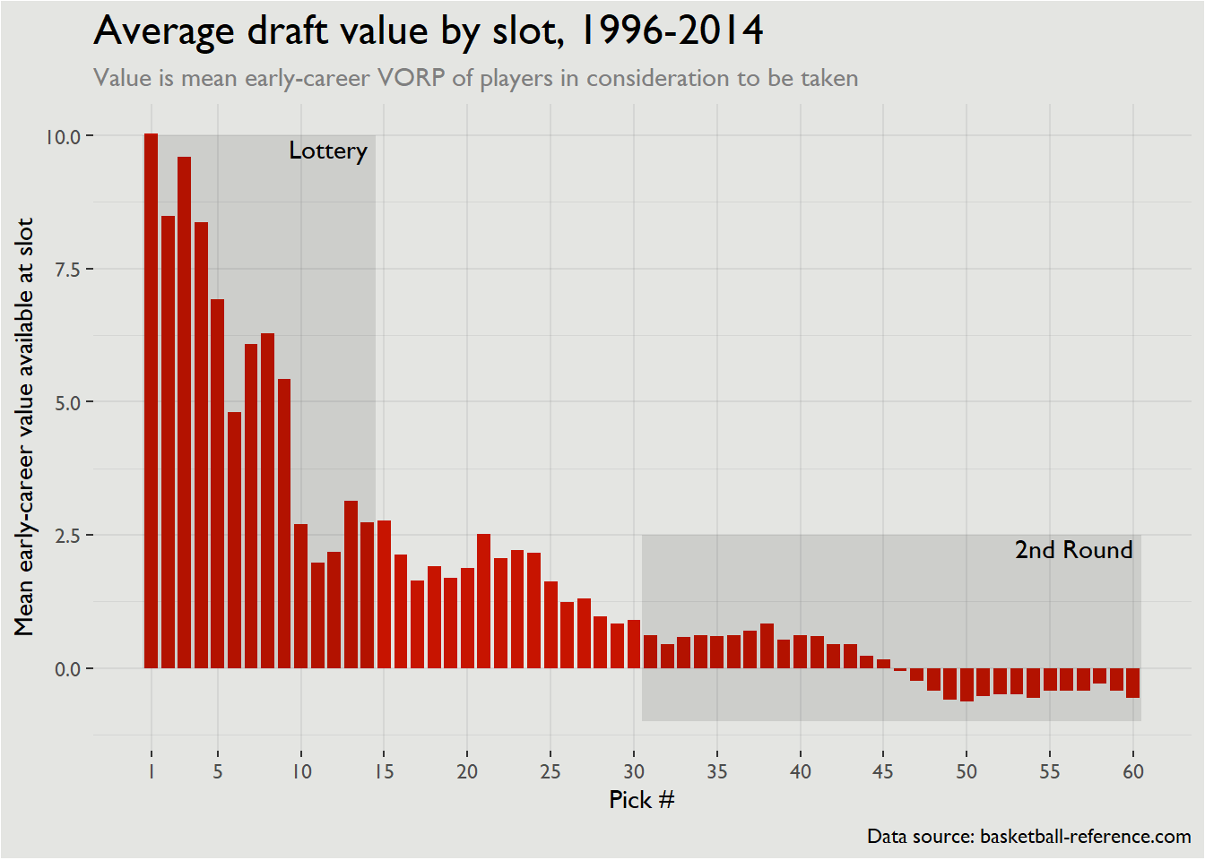
Takeaways
A couple of things jump out immediately:
- There’s a big drop-off in value towards the back half of the lottery. This specifically occurs after the 9th pick, but I’d be cautious about applying that as a principle to specific drafts. The general principle that starter-quality rotation players will be clustered in the top 10 picks holds though. This suggests that NBA executives should be more willing to do top-10 protection on draft picks instead of lottery protection, particularly for drafts well into the future.
- There’s not much difference between late firsts and early seconds. This is turning into a bit of conventional wisdom, but it’s nice to see confirmation here. The difference in value between first-round picks in the late 20s and second-rounders is pretty minimal, and is likely offset by the additional contractual flexibility GMs get with second-rounders. This holds true down to about the mid-40s, when players value rapidly drops off.
Further exploration
There are a couple of questions I’d still like to be able to answer on expected outcomes in the draft, like the chance of getting a starter/rotation player at each point in the draft, but I’m happy with this analysis and feel confident that next time I’m wondering what the average value of N pick is, I have somewhere easy to look it up. Let me know if you have any comments or ideas for me!
Glad to know Nikola Jokic is the third-best defender in the NBA, just behind Jae Crowder and ahead of Rudy Gobert!↩︎
Whether as an on-court player, or in terms of trade value, pick return, etc.↩︎
The contract for first-round picks is a standard 2+2 (two years with two one-year team options at the end).↩︎
I will never pass up the opportunity to post this video.↩︎